A discussion this week about comparitive strengths of schedule led me to ponder how to formulate the question from composite ranks. The usual SOS measurement for a particular computer rating is just the average value of opponents' ratings. Average ranks in that case are not really indicative for a specific rating, since rating values are more spread out on the tails of the curve than the difference in ordinal ranks.
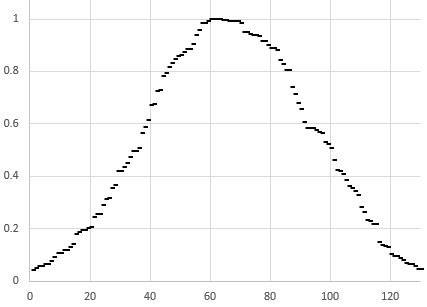
We have only the ordinal ranks for the 100+ computers in Massey Ratings College Football Ranking Composite as of Sat Oct 26 06:58:59. A proxy for a composite value can be found in the consensus rank by Borda Count, since we have the values by which the ranks are defined. The distribution is at least similar to what we'd expect from an advanced rating's values. With μ = 664.135 and σ = 3704.711 we see that ℯ-((x-μ)⁄σ)2 approximates a normal curve.
So we can use opponents' Borda count to define an SOS based upon a composite ranking.
The next question is why should we care about SOS anyway? All of the advanced ratings apply their version of SOS to derive their ratings to begin with. A technical answer is that the directed games graph is so weakly connected that comparison based upon records vs common opponents isn't possible. Advanced ratings produce their rankings based upon A→B→ chains as long as needed to form the comparisons but this results in a necessarily fuzzy measurement.
To demonstrate that we'll use our proxy rating. Tier 1 is the #1 team. Tier 2 consists of the #2 team plus all the teams that are as close to number #2 as #2 is to #1. Tier 3 is topped by the first team not in tier 2 and includes all teams as close to it as it is to the top of tier 2, and so on. With 45 computer rankings for games through 26 October, the process comes up with
(The breakdown will be different as more of the 100+ computers contribute to this proxy rating.)
Cutoff Tier Ranks Teams 5797 1 1 { Ohio State } 5621 2 2-5 { LSU; Clemson; Penn State; Alabama } 5189 3 6-14 { Auburn; Oregon; Florida; Oklahoma; Utah; Baylor; Wisconsin; Michigan; Georgia } 4853 4 15-21 { Cincinnati; Minnesota; Iowa; SMU; Appalachian State; Notre Dame; UCF } 4383 5 22-33 { Boise State; Washington; Memphis; Navy; Iowa State; Kansas State; Air Force; Southern California; Texas A&M; Texas; Oklahoma State; Wake Forest } 3731 6 34-43 { Michigan State; Indiana; TCU; Virginia; Louisville; Arizona State; Pittsburgh; UL Lafayette; San Diego State; Florida State } 3211 7 44-55 { Utah State; North Carolina; Missouri; Washington State; Tulane; Stanford; Wyoming; Kentucky; Mississippi State; Duke; South Carolina; Florida Atlantic } 2660 8 56-70 { Louisiana Tech; Miami-Florida; California; UCLA; Hawaii; Nebraska; BYU; Temple; Tennessee; Virginia Tech; Arizona; Illinois; Marshall; Boston College; Georgia State } 2113 9 71-86 { Oregon State; Texas Tech; West Virginia; Western Michigan; Mississippi; North Carolina State; Colorado; UAB; Southern Miss; Houston; Georgia Southern; Western Kentucky; Tulsa; South Florida; Arkansas State; Miami-Ohio } 1530 10 87-96 { Maryland; Fresno State; Syracuse; Ohio; Purdue; Ball State; Toledo; Kansas; Northwestern; Buffalo } 956 11 97-114 { Middle Tenn State; UL Monroe; Eastern Michigan; Georgia Tech; Nevada; San Jose State; Central Michigan; Arkansas; Army; Northern Illinois; Vanderbilt; Liberty; Coastal Carolina; Florida Intl; North Texas; Troy; Colorado State; Kent State } 126 12 115-127 { UNC-Charlotte; Texas State; Rutgers; East Carolina; UNLV; Texas-San Antonio; New Mexico; Connecticut; Bowling Green; Rice; South Alabama; Old Dominion; New Mexico State } -577 13 128-130 { UTEP; Massachusetts; Akron }
So the notion that SOS can provide context for comparing teams in the same tier makes sense. The next question is how to present SOS data in a useful way. I decided to produce a report with a one-line "resume" for each team, listing the opponents' ranks separately for the teams' wins and losses ordered by the average openents rating for wins-only (a team could easily have the highest SOS and finish 0-12.)
For our tier-3 teams, the report looks like this:
Strength of schedule based upon the average computer rankings of teams' opponents. Ordered by average opponent rank in teams' wins.The opponents' ranks for wins are ordered best-to-worst and losses worst-to-best. The temporal and location contexts are provided by links from the team names to what I call the resume view of their schedules.
Rank Borda Team SOS Rank Rank SOS(W) Wins Losses 6 5449 Auburn 3773 6 7 3183 7 30 48 52 104 114 8 2 7 5400 Oregon 3030 36 17 2685 23 47 49 58 77 101 131 6 13 5240 Michigan 3373 20 19 2679 17 20 67 97 105 117 12 4 12 5254 Wisconsin 3039 35 24 2621 13 34 84 95 103 114 67 1 8 5377 Florida 2980 43 25 2590 6 51 54 57 64 131 131 2 10 5288 Utah 2742 61 27 2484 39 47 58 62 71 106 131 29 11 5264 Baylor 2439 78 32 2439 26 27 32 72 120 124 131 14 5189 Georgia 2537 70 33 2421 20 51 64 85 107 131 54 9 5352 Oklahoma 2680 65 35 2403 31 59 72 73 80 94 131 27
I will add the report to the Ranking Analysis section of the home page, and its current version will always be at http://football.kislanko.com/2019/borda_sosW.html.