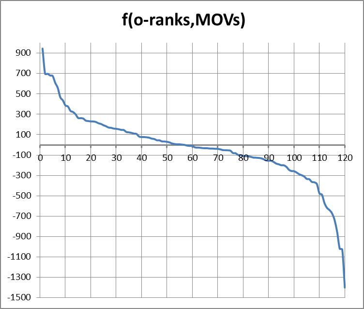
The horizontal axis is meta-rank, the vertical is the meta-rating.
I am fond of inventing meta-rankings ("ratings" whose inputs are other rankings instead of game results) not because they have any intrinsic value, but because they make visible characteristics of the input rankings that aren't otherwise obvious. I'm especially fond of meta-rankings that turn ordinal ranking data into a rating value, because good variations of those can show that the difference between #1 and #10 is a lot greater than that between #56 and #64.
In fact, the meta-rating described below has a larger difference between #1 and #2 than between #40 and #80, as you can see from the graph:

The horizontal axis is meta-rank, the vertical is the meta-rating.
|
For winning teams, the MOV factor is capped at three scores - we don't learn more about the winner as the margin goes up past that. The negative MOV factor for the losing team is not capped because we do get more information about a team that loses by 10 scores than one that loses by three.
For each game, multiply the three factors, then take the average over all games to form the "rating."
Now, this isn't more of a good "rating" than any other meta-rating, but it is useful in the same way I think the baseball RPI is. I don't think it is a great measure of team performance, but it's as reasonable as any as a sort sequence. Here's a sample:
| Meta Rank | ƒ(ranks) | Rank | Team | Rec | Conf | Best Win | Other Wins Over | Worst Loss | Other Losses To |
|---|---|---|---|---|---|---|---|---|---|
| 1 | 944 | 2 | Alabama | 5-0 | SEC | 16 | 20 30 102 106 | – | |
| 2 | 700.4 | 8 | Clemson | 5-0 | ACC | 20 | 24 35 76 121 | – | |
| 3 | 698.2 | 4 | LSU | 5-0 | SEC | 13 | 22 60 84 121 | – | |
| 4 | 679 | 4 | Oklahoma | 4-0 | B12 | 35 | 42 55 73 | – | |
| 5 | 676.5 | 6 | Boise State | 4-0 | MW | 34 | 55 62 64 | – | |
| 6 | 608.25 | 6 | Oklahoma State | 4-0 | B12 | 28 | 55 59 73 | – | |
| 7 | 558 | 8 | Michigan | 5-0 | B10 | 22 | 40 50 90 107 | – | |
| 8 | 540.75 | 10 | Texas | 4-0 | B12 | 38 | 58 65 94 | – | |
| 9 | 437.4 | 7 | Wisconsin | 5-0 | B10 | 17 | 87 102 103 121 | – | |
| 10 | 393.75 | 6 | Stanford | 4-0 | P12 | 65 | 70 73 91 | – | |
| 11 | 360.4 | 22 | Notre Dame | 3-2 | ND | 31 | 41 88 | 29 | 8 |
| 12 | 334.2 | 23 | Arizona State | 4-1 | P12 | 32 | 42 103 121 | 16 | |
| 13 | 325.4 | 17 | South Carolina | 4-1 | SEC | 34 | 49 67 90 | 20 | |
| 14 | 300.8 | 17 | Nebraska | 4-1 | B10 | 26 | 71 88 121 | 7 | |
| 15 | 268.8 | 32 | Southern California | 4-1 | P12 | 47 | 60 73 107 | 23 | |
| 16 | 263.4 | 26 | Washington | 4-1 | P12 | 45 | 47 68 121 | 17 | |
| 17 | 262.8 | 16 | Illinois | 5-0 | B10 | 23 | 50 76 76 121 | – | |
| 18 | 258.6 | 41 | Pittsburgh | 3-2 | BigE | 29 | 110 121 | 38 | 22 |
| 19 | 238.75 | 28 | Texas A&M | 2-2 | B12 | 42 | 110 | 20 | 6 |
| 20 | 234.25 | 13 | Oregon | 3-1 | P12 | 64 | 73 121 | 4 | |
| 21 | 229.6 | 16 | Florida | 4-1 | SEC | 33 | 84 108 116 | 2 | |
| 22 | 225.25 | 33 | Tennessee | 3-1 | SEC | 46 | 110 121 | 16 | |
| 23 | 215.4 | 14 | Georgia Tech | 5-0 | ACC | 28 | 76 82 104 121 | – | |
| 24 | 205.5 | 40 | San Diego State | 3-1 | MW | 56 | 88 121 | 8 | |
| 25 | 193.25 | 21 | Kansas State | 4-0 | B12 | 33 | 52 102 121 | – |
Here the input Rank is itself a meta-rank: it is the best rank for which >50% of the computer rankings tracked by Dr. Massey rank the team at least that highly. It's kind of interesting to look at the Rank→Meta-Rank changes for each team, and the presentation makes it easier to see why one team's results against their schedule give it a different result than another's against their schedule (for this input Rank.)
The team-names link to the better-wins/worse losses tables for each of the teams. The "Valu" column combines the opponent's rank and MOV (but not the bonus.)
One of the things I like about the report is that the opponents' names do not appear. It's easier for us humans to be objective when we see only the opponents' rankings, not their names. Here's the full report.